
Value at Risk (VaR) is a commonly used measure of market risk in portfolios. VaR is formally defined as the ‘predicted loss at a specific confidence level over a given holding period’. The Basel II accords require a 99% confidence level over a ten-day period while South African hedge fund regulations (BN52) require a 99% confidence level over a one-day period.
While the methodology behind VaR has been around for several years arguably the most notable advancement of VaR was by J.P. Morgan in the early 1990’s. J.P. Morgan CEO Dennis Weatherstone famously called for a “4:15 report” that combined all firm risk on one page, available within 15 minutes of the market close, this led to the creation of their RiskMetrics system and global recognition of the VaR methodology.
There are generally three accepted approaches to measuring VaR:
- Variance-covariance – assumes the normal distribution of returns and uses statistical measures, mean and standard deviation, to determine the VaR,
- Historical simulation – uses historical returns to determine the VaR, and
- Monte Carlo simulation – uses randomly generated returns to determine the VaR.
Statpro Revolution** uses the Historical simulation methodology because of its ability to accommodate all asset classes as well as their derivatives and the methodology is intuitive.
Practical Example:
Based on a simple equity portfolio.
Before generating the VaR, we select the Confidence Level, Holding Period and History.
 The Confidence Level is used to specify the applicable loss, if 500 returns were observed, a Confidence Level of 99% would imply the 495th worst return, based on today’s market value, would represent the VaR.
The Holding Period specifies the return interval, One Day would imply the return over one day.
The History refers to the number of observations. Two Years implies approximately 500 observations or days where returns were observed in the market (One Year is approximately 250 trading days).
Some things to remember:
- Using a One Week Holding Period would imply only 245 observations in one year, with each return being based over one week (five trading days).
- The Portfolio’s VaR represents a particular “day” and the individual security returns on this “day” contribute to this Portfolio VaR. The Portfolio VaR is not the summation of the individual securities VaR.
- The historic correlation (beta) relationship is implicit in the Historical simulation methodology.
Below is the histogram of the observations (daily over two years, approximately 500 observations):
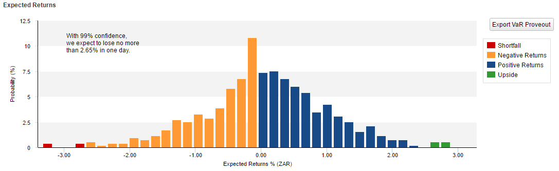 From the above the distribution is clearly not normal as per the assumption of the variance-covariance methodology.
The Portfolio Risk is displayed on the top, indicating that the Portfolio could lose 2.65% of its market value at the 99% Confidence Level over One Day.

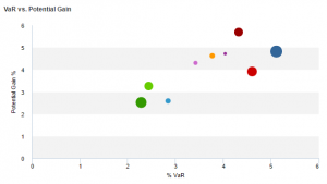
On the left is an ex-ante VaR versus Potential Gain graph at sector level, this can be equated to the ex-post Risk versus Return graph. In the classic sense, we require the highest potential return for the least risk.
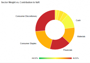
On the left is the Sector Weight versus the Contribution to VaR, here we are comparing the weight of the sector (size) to its contribution to VaR (colour).
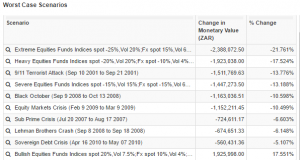
On the left are various stress tests performed on the Portfolio over historic periods or simulated conditions. Unlike VaR these represent the Worst Case Scenarios over the historic period.
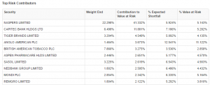
On the left are the Top Risk Contributors, these are the biggest contributors to the Portfolio VaR.
As is to be expected to get accurate VaR outputs the individual securities must be correctly loaded, for example options must be loaded with the correct option characteristics (e.g. American/European, call/put, strike, expiry date) to generate a synthetic history for VaR purposes.
Although VaR has achieved global recognition it still has its’ limitations and critics, for example:
- Nassim Taleb (2007) highlighted the reliance on shorter time periods, model limitations and the technical impossibility to estimate the risks of rare events which VaR purports to do.
- David Einhorn (2008) highlighted that VaRs’ usage has led to excessive risk-taking, focused attention on the manageable risks near the centre of the distribution and ignores the tails, creates an incentive to take “excessive but remote risks” and was “potentially catastrophic when its use creates a false sense of security among senior executives and watchdogs”.
Being cognisant of the above means we should not place an inordinate degree of faith in VaR as if it were a magic number that tells all about a Portfolio’s risk, but rather use VaR as one of many tools in a risk professional’s arsenal to manage and hence mitigate risk.
** The example above was performed in Statpro Revolution and I am grateful for the assistance they provided.
For more information please use the links below:
https://revolutionsupport.statpro.com/hc/en-us/articles/229174307-Value-at-Risk-VaR-
http://www.nytimes.com/2009/01/04/magazine/04risk-t.html?pagewanted=1&_r=1